Setup
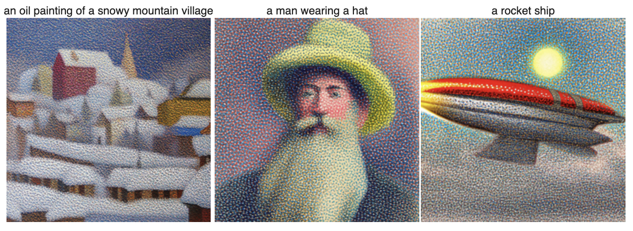
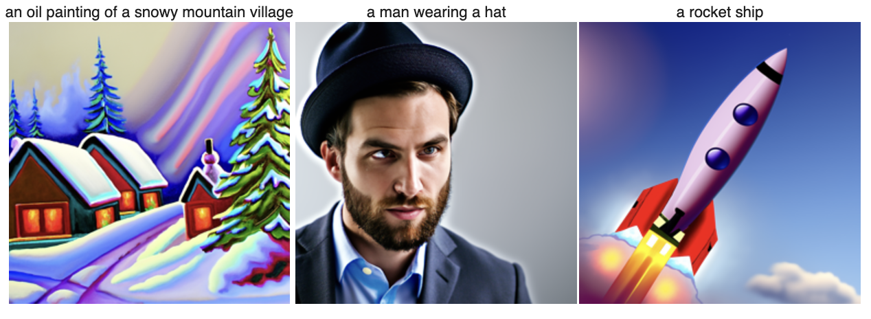
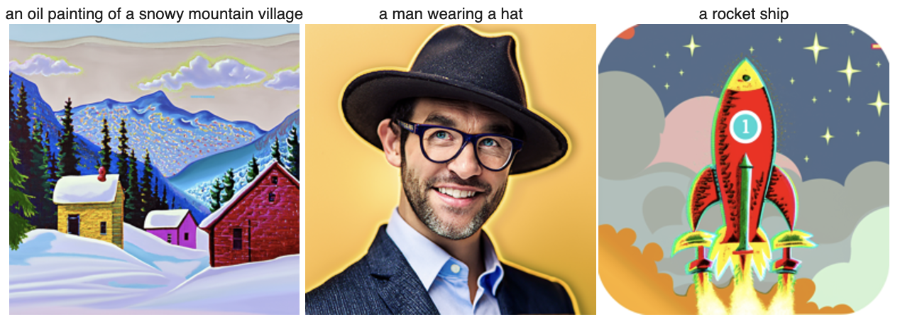
For this project, I downloaded the DeepFloyd IF diffusion models from HuggingFace. We instantiate 2 stages. Below are some initial testing of the model with inferences=[5, 20, 50] on a series of prompts.
1.1 Implementing the Forward Process
We implement the Forward Process equations to add noise to clean images. Here are some outputs for noise levels [250, 500, 750].

250

500

750
1.2 Classical Denoising
In classical methods, we usually denoise image by applying a gaussian filter. Here are the corresponding outputs. As you can see they are not very effective in restoring the original image.

250

500

750
1.3 One-Step Denoising
Using a pretrained diffusion model, we attempt to denoise the noisy images. For the 3 noisy images at t=[250, 500, 750] we ask the UNet to estimate the noise. We then subtract this estimated noise from our noisy image to obtain an estimate of the original image. During this process, we need to scale the noise according to specific coefficients for each timestep. Here are some of the results. They are not bad, but for extremely noisy images, we get a rather blurry estimate in the output, let's see if we can do better.

250

500

750
1.4 Iterative Denoising
For really noisy images, we want to improve the quality of our outputs, so now we will try iterative denoising. We use a slightly different equation and iterate our denoising for a give t > 0 all the way down to t=0 (our clean image). The advantage of iterative denoising is that we gradually reconstruct images by remove noise over mulitple steps, this added conputation results in fine-grain estimation and noise removal. Here are the better results!

t=900

t=840

t=690

t=540

t=390

t=240

t=90

t=0 : Final Denoised Image

One Step

Blurry Gaussian
1.5 Diffusion Model Sampling
Using our iterative denoising function from above, we will use randomly generated noise to create brand new images. We denoise from the highest noise value (t) and try to obtain a new clean image at t=0. Here you can see a random sample of 5-newly generated images.

Sample 1

Sample 2

Sample 3

Sample 4

Sample 5
1.6 Classifier-Free Guidance (CFG)
The generated images above are quite good, but some of them do not make too much sense. So we will try a technique called Classifier-Free Guidance. We follow the formula below to update our noise estimates. We run the iterative denoise function on this new noise estimate and now we have a new set of 5 samples, that are fictional yet sensible.

Iterative Denoise CFG Sample 1

Iterative Denoise CFG Sample 2

Iterative Denoise CFG Sample 3

Iterative Denoise CFG Sample 4

Iterative Denoise CFG Sample 5
1.7 Image-to-image Translation
Here we want to take our original test image, add a little noise and then iteratively denoise them back to our original image. The really cool thing here is that with a lot of noise, our iterative denoising might return completely new images or new images that resemble our original image's most prominent features. This exhibits the model's ability to hallucinate features of a noisy image.


1.7.1 Editing Hand-Drawn and Web Images
We want to explore the model's "creative" abilities, by using 1 image from the web, and 2 Hand-Drawn images. We will add a little bit of noise to the images we have obtained and then see how the model can create new images, and recreate different versions of our original image.


1.7.2 Inpainting
We are now going to explore a diffusion model's ability to modify specific features of an image. We try to do this by masking our original image and telling our algorithm to only noise a certain part of the image, keeping the rest of the image exactly the same. Now we ask the diffusion model to denoise the noisy portion of the masked image, and then we recompose the images to obtain a slightly altered feature in our original image.


1.7.3 Text-Conditional Image-to-image Translation
We know want to modify our images based on our prompts. We use our noisy test image and utilize a different prompt to see how the model iteratively denoised the image based on the prompt to obtain intesting morphs of the test image to the prompt specifications.
"A rocket ship" -> picture of Campanille


"A pencil" -> picture of giraffe


"a photo of a dog" -> picture of dolphin


1.8 Visual Anagrams
For visual anagrams, we use two UNets with different sets of prompts. For the first UNet we set it up as we have done previously with a new prompt. However, for the second UNet we flip our original noisy image and pass that as input along with a brand new prompt. We flip back the second denoised image and average it with the first denoised image to obtain our new starting point image. We then apply our formal diffusion techiques on the new averaged image to obtain the visual anagram effect.
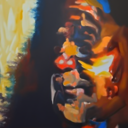
an oil painting of an old man
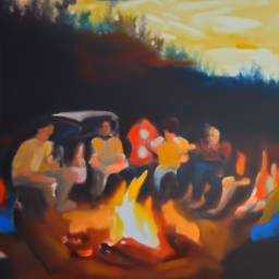
an oil painting of people around a campfire
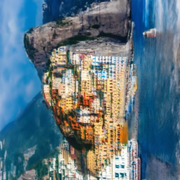
a photo of a man
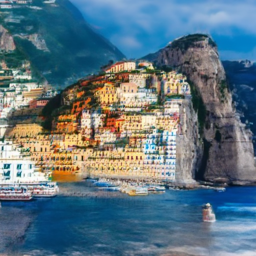
a photo of the amalphi coast
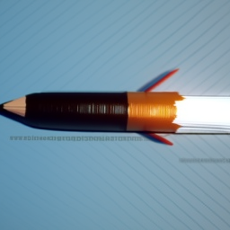
a pencil
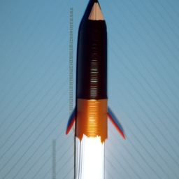
a rocket ship
1.9 Hybrid Images
For the hybrid images, we use the same workflow as the visual anagrams, but with a different equation. We take the denoised images for two different prompts. We then apply a low-pass and high-pass filter to the first and second denoised images, respectively. We then add the filtered images together to create our new starting point image. We then apply our formal diffusion techiques on the new filted image to get our Hybrid Image.

A Skull and Waterfalls

A man and snowy mountains

A rocket ship and Waterfalls
Part B: Diffusion Models from Scratch!
Obtaining a low-level understanding of Diffusion Models!
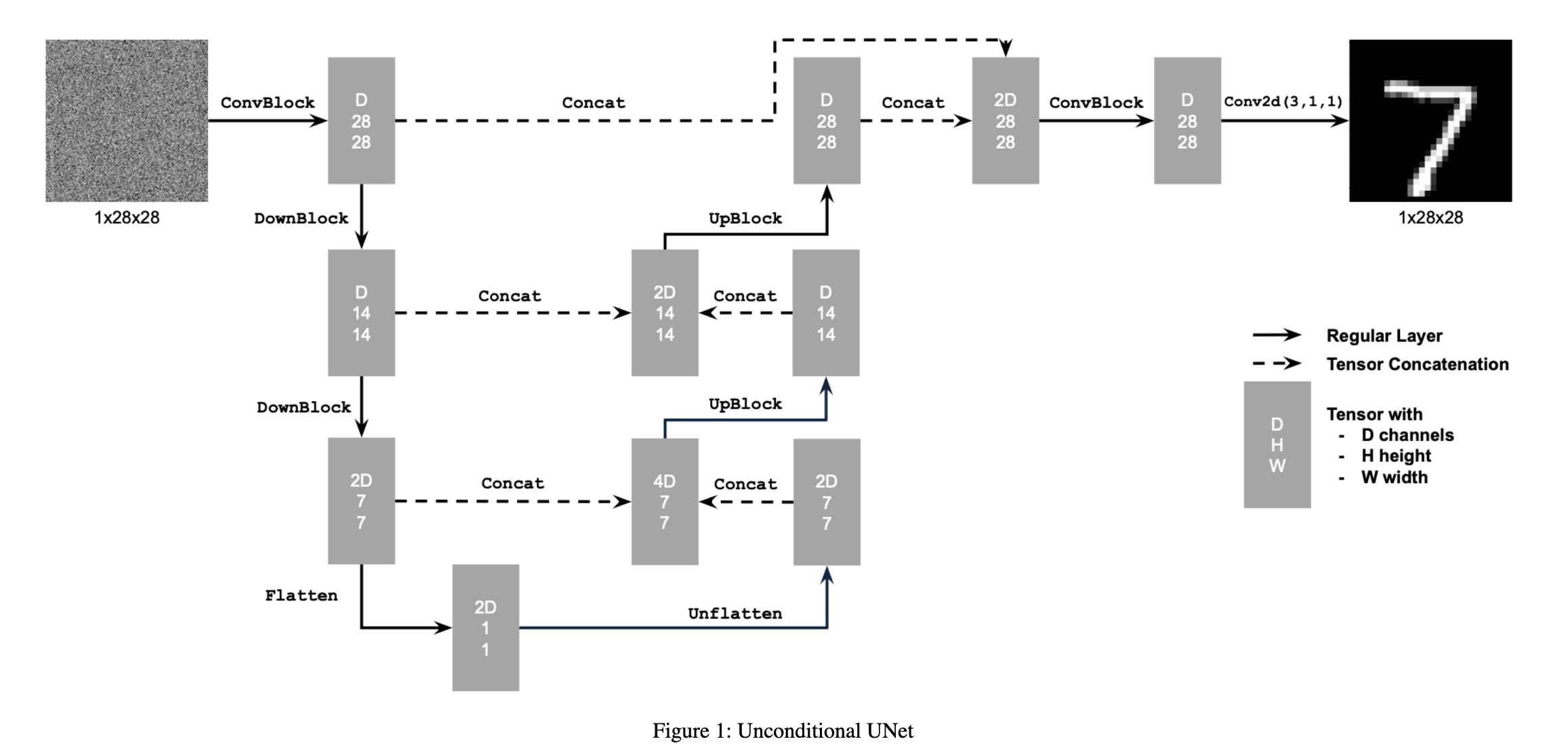
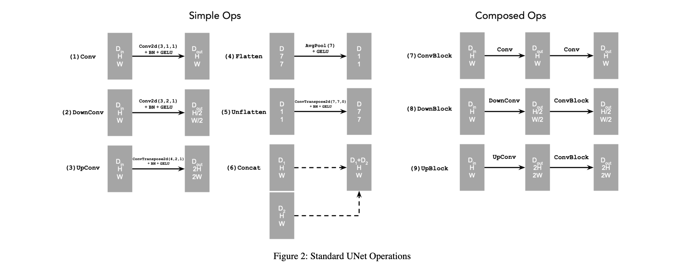
1.1 Implementing the UNet
UNets are used to denoise images. We use the UNet architecture below to capture both local and global features. We use various techniques and a pretty deep architecture to create a roboust UNet model.
1.2 Using the UNet to Train a Denoiser
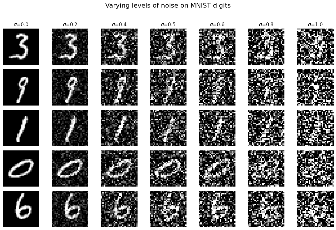
Here is a visual of the different noising processes over a range of epsilons.
1.2.1 Training
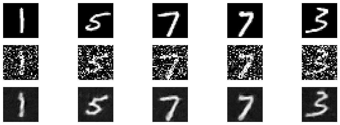
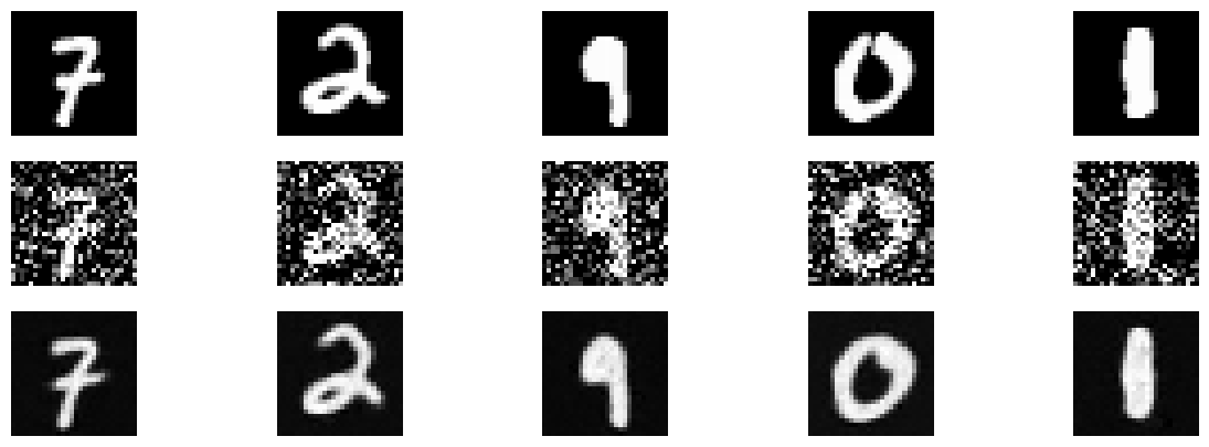
We train our UNet on the noised MNIST dataset. We use D=128 as our hidden dimension, and train our UNet for a noise of epsilon=0.5.


We also visualize the denoised output after the 1st and 5th epochs.
1.2.2 Out-of-Distribution Testing
Upon completing training of the UNet for epsilon=0.5, we sample the UNet with varying levels of noise (epsilon values) to see the robustness of the model's outputs.


2.1 Adding Time Conditioning to UNet
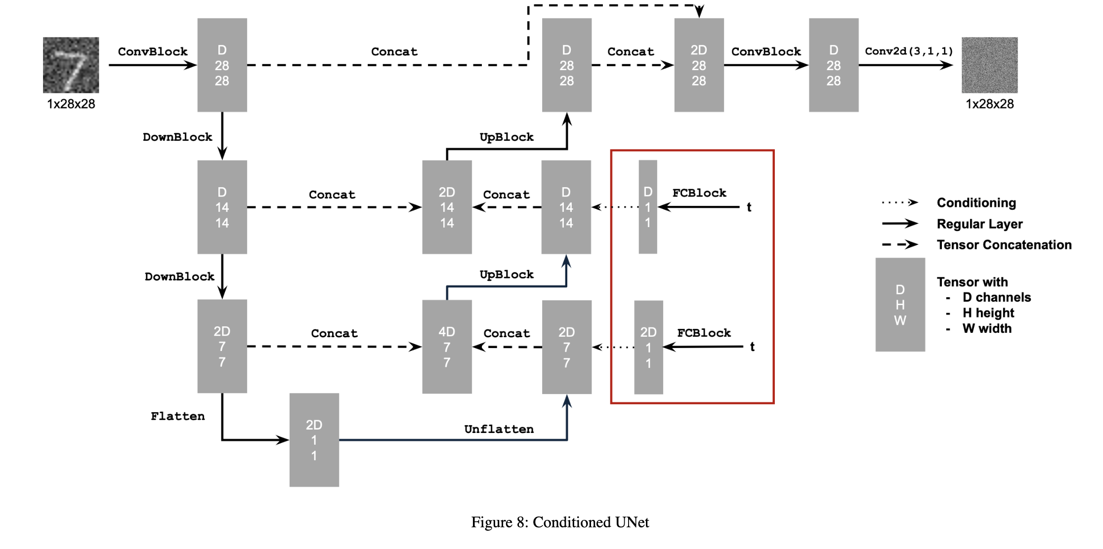
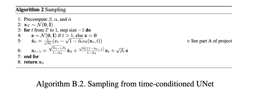
Now that we have a UNet, we implement a DDPM to iteratively denoise images, and add Time Conditioning to the model's capabilities. The big difference now, is that the model is now trained to predict noise rather than the clean images, it is also now taking in as input a noisy image and a t parameter at which the clean image was noised by the forward process. Now, instead of training UNets for seperate noise levels it is conditioned on timestep t. This should make it robust to different timesteps of noise and provide robust outputs.

2.2 Training the UNet
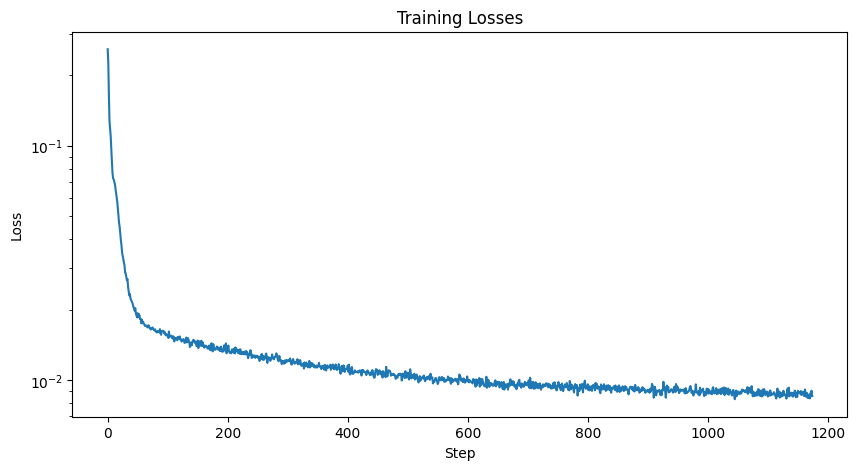
We train the UNet of L2 loss gradient descent. Here is a visualization of the training loss curve.


2.3 Sampling from the UNet
We now sample the UNet to see how good our model reacts to varying levels of noise. Let's sample at epochs 5 and 20 to visualize the model's effectiveness.
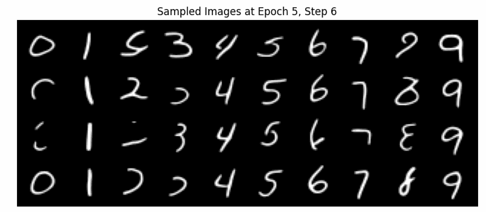
Epoch 5
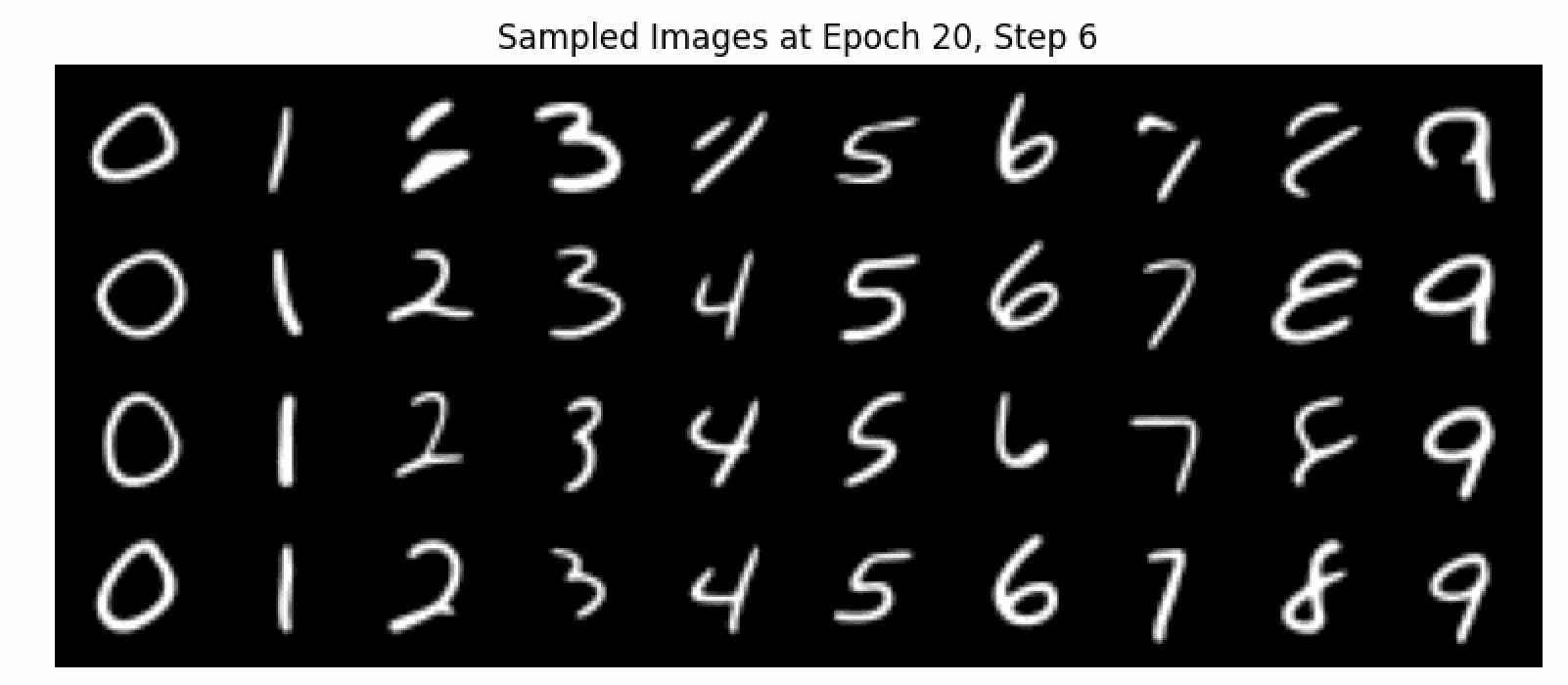
Epoch 20
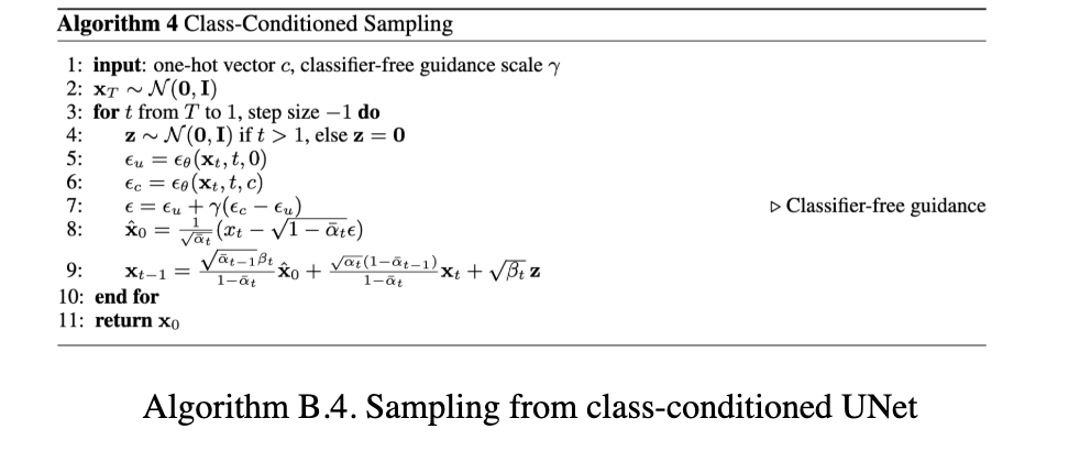
2.4 Adding Class-Conditioning to UNet
We now want to improve our model by introducing Classifer Free Guidance. We use a gamma=0.5 for this part. Here is a visual of the training loss curve.
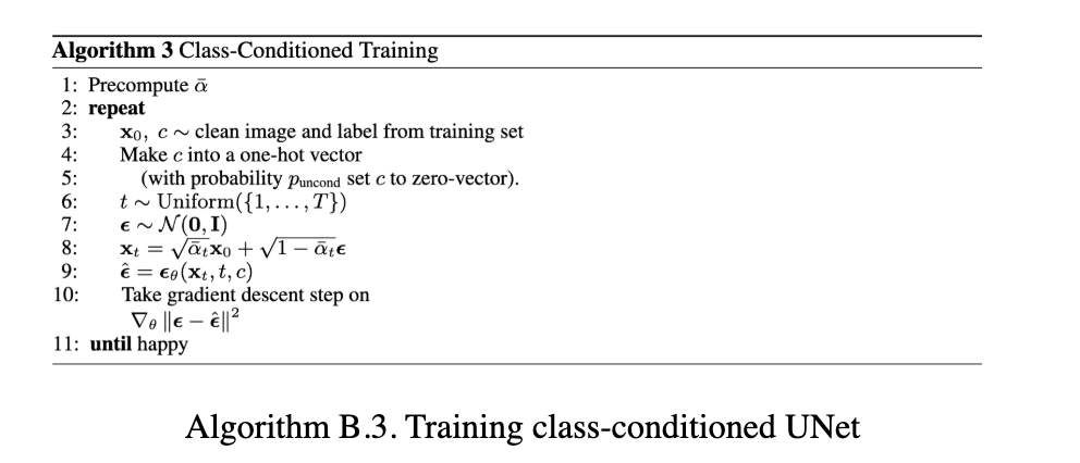

2.5 Sampling from the Class-Conditioned UNet
We now sample the UNet to see how our model performs to various digits. Let's sample at epochs 5 and 20 to visualize the model's effectiveness.
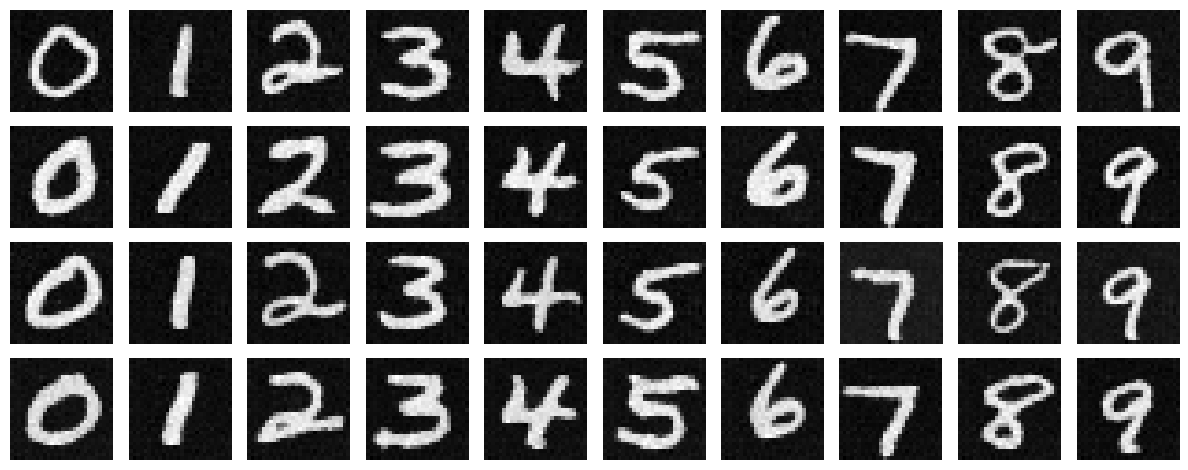
Epoch 5
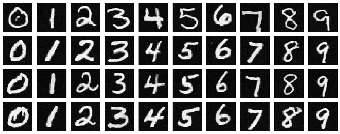
Epoch 20